CoeViz Documentation

Index

About CoeViz

Terms of use and disclaimer

References to cite the server

Methods

Implementation

Covariance and conservation metrics

Manual

Header

Tree Diagram

Heatmap

Navigation Pane

Circular Relationship Diagram

Example

Acknowledgements

About CoeViz

CoeViz is a web-based tool for analysis and visualization of coevolution of protein residues. The server computes pairwise coevolution scores using three metrics: Mutual Information, Chi-square Statistic, and Pearson correlation. Also, an option for computing conservation scores based on the Joint Shannon Entropy is provided. Interactive analysis includes dendrogram of clustered residues (hierarchical cluster tree), zoomable heatmap, circular diagram of inter-residue relationships, scatterplot of multi-dimensional scaling (MDS), and the mapping of residue clusters to a protein sequence or 3D structure. The tool is part of the POLYVIEW-2D protein structure visualization server and available from the resulting pages of POLYVIEW-2D.

Terms of use and disclaimer

All images generated by the CoeViz server can be FREEly saved, printed, and distributed by means of any media without our written permission for academic and non-commercial purposes. However, the use of CoeViz pictures SHOULD be acknowledged by a reference to the server.

The use of the CoeViz server is at your own risk and no liability is accepted for any loss or damage arising through the use of the web site and protein annotations generated by the server.

References to cite the server

F.N. Baker and A. Porollo (2016) CoeViz: a web-based tool for coevolution analysis of protein residues. BMC Bioinformatics, 17: 119.

F.N. Baker and A. Porollo (2018) CoeViz: A Web-Based Integrative Platform for Interactive Visualization of Large Similarity and Distance Matrices. Data, 3: 4.

Methods

Implementation

Unless the multiple sequence alignment (MSA) for a given protein is provided by the user, alignments are generated on the server side using three iterations of PSI-BLAST with the profile-inclusion threshold of expect (e)-value = 0.001 and the number of aligned sequences 5000. The sequence homology search can be done against Pfam, NCBI NR, or UniProt (default) databases. The NR database is available with three options: full and reduced to 90% or 70% sequence identity by CD-HIT. The UniProt is avilable with two options: reduced to 90% (default) and 50% sequence identity, as provided by UniProt. Interactive analysis and visualization include: cluster tree, zoomable heat map, relationship circular diagrams, and MDS scatterplots.

Covariance and conservation metrics

Coevolution scores are computed from the MSA using three different covariance metrics: mutual information (MI, Eq. 1), chi-square statistic (χ², Eq. 2), and Pearson correlation (r, Eq. 3). Conservation is defined by the joint Shannon entropy (S, Eq. 4). Each metric, in turn, is computed using four weighting schemes: weighted by sequence dissimilarity or sequence gapping in the alignment (Eqs. 5 and 6), by phylogeny background (Eq. 7), and non-weighted. MI scores have an additional adjustment using the average product correction (APC, Eq. 8) to produce MIp scores (Eq. 9).

All metrics based on frequencies are computed using four states as possible combinations of amino acids at two positions (i and j), where each amino acid is either equal (X) or not equal (!X) to the one in the query sequence.

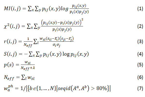
where x={X; !X} and y={Y; !Y}; p(s) is the observed frequency of state s={x; y; x,y}; N_eff is the effective sum of weights of alignments where both positions are not gaps. w_sl is a weighted count of state s, which is equal to 1 for non-weighted scores, 1–(percent of sequence identity) or 1–(percent of gaps) of the alignment l for weighting by sequence dissimilarity or alignment gapping, respectively, and w_a^ph for weighting by phylogeny. w_a^ph is a weight for sequence A^a in the MSA of N total sequences that equals to one over the number of sequences A^b in the MSA that have at least 80% sequence identity to A^a. s_il is a similarity score that quantifies the change of an amino acid at position i to the one in the aligned sequence l. s¯_l and σ_i are mean and standard deviation, respectively, of all similarity scores of changes for a given position represented across the all sequences aligned to the query. Similarity scores are taken from the position specific similarity matrix (PSSM) generated by PSI-BLAST. λ is a pseudo count, which is equal to 1 for all metrics here.

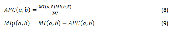
where MI(a,x¯) is the mean MI of column a, and MI¯¯ is the overall mean MI.

Negative values of MIp scores are assigned to 0, and then all MI scores are min-max normalized to range [0, 1]. S is normalized to the same range by factor 1/log (4). χ2 values are converted to the corresponding cumulative probabilities at degree of freedom (df) = 1.

Scores for each metric are organized in symmetrical matrices with the main diagonal presenting plain or weighted frequencies, as defined above, of each individual residue for MI-and χ2-based metrics, and the individual Shannon entropies using 20 states (20 amino acids) for S-based metric. Individual entropies are computed using probability part of the PSSM files from the PSI-BLAST output and normalized to range [0, 1] by factor 1/log(20). Residues of the query protein are clustered using hierarchical clustering with the complete linkage method. Prior to clustering, negative r scores are assigned to 0; MI, r, and χ2 scores are converted to distances by 1–score transformation.

Manual

The CoeViz layout is split into 4 main panes: the header, tree diagram, navigation pane, and heatmap. Additional pane is shown upon request for a given cell of the heatmap. It presents inter-residue relationships using an interactive circular diagram. Detailed decription of the panes follows below.

1. Header

   Use the header to select which coevolution metric to use for analysis. Currently computed metrics include: Mutual Information (MI), Chi-square Statistic (Chi²), Pearson correlation coefficient, and Joint Shannon Entropy (JSE). Each metric, in turn, is available with plain values or weighted values. The weights are used to diminish contribution to the scoring by homologous sequences similar to the query protein. The default (first to display) coevolution metric is a weighted chi-square statistic.

   Once metric and weighting scheme are selected from a dropbox, other panes will be automatically updated accordingly.

2. Navigation Pane

   The navigation pane spans the right side of the browser window below the header. At the top of the navigation bar there is a group of buttons.

   • The zoom in and zoom out buttons increase or decrease the zoom levels on the heatmap, respectively.
   • The export button brings up a menu enabling download of the sequence alignments file, coevolution data in tab-separated text format, cluster dendrogram image file, and current view of the heatmap.
   • The toggle labelling button can be used on certain zoom levels to change the type of information displayed as text in each cell. There are three different labels for display: (1) heatmap cell coordinates (row and column indexes), (2) positions of residues in the protein sequence (depending on the input, e.g. a PDB structure, residue positions may be numbered differently, or non-consecutively, than the heatmap cell indexes), and (3) computed score according to the chosen metric and weight.
   • The help button displays a quick reference on how to use CoeViz.

   Below the buttons, there is a miniaturized version of the heatmap, which can be used to navigate to specific places on the heatmap by dragging the yellow box or by clicking on a specific point in the miniature heatmap.

   Below the miniature heatmap navigation tool is a quick view of the current cell, that is, the cell the mouse is currently over. If the mouse is moved out of the heatmap, the current cell view will stay on the last displayed cell. This tool displays the heatmap coordinates, residues labels and positions, and computed score for each cell.

   In order to quickly jump to residues of interest, there is a Center View on Cell tool directly beneath the Current Cell view tool. This will center the heatmap view on the cell specified by the row and column numbers, and highlight it briefly (for a reference) with a yellow box that fades.

3. Tree Diagram

   The diagram shows an interactive image of the cluster tree generated using the complete-linkage hierarchical clustering algorithm based on a given metric. In case of Chi² and MI, the scores are converted to distances by 1-score transformation. In case of Pearson, distances are 1-abs(score).

   Each leaf of the tree diagram has a colored circular label indicating hydropathy according to the conventions previously established in POLYVIEW-2D. The branching points of the tree are clickable to highlight a chosen cluster. Clicking on a leaf causes Heatmap, Circular Diagram, and MDS plot to update by focusing on a newly chosen residue. The tree is scrolled automatically to focus on a residue chosen in other panes.

4. Heatmap

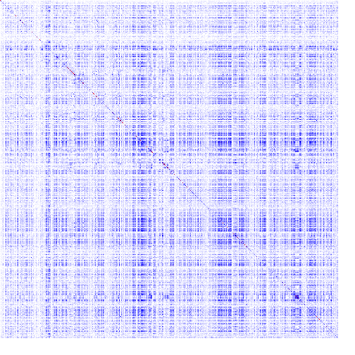
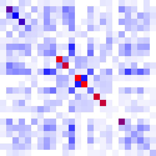
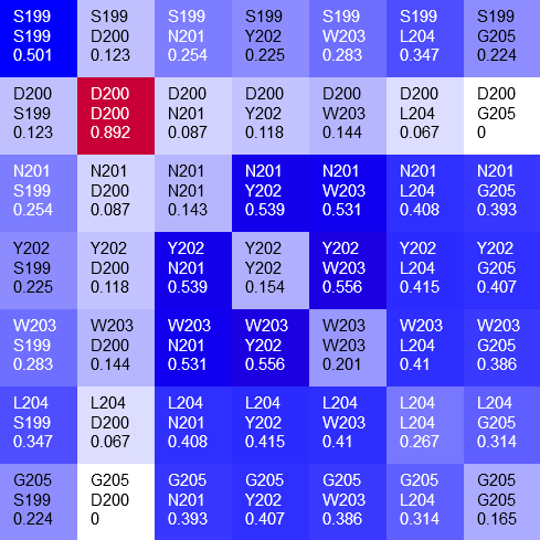
   The heatmap is a color-based representation of coevolution scores. White through blue to red color gradient represents no covariance through moderate to strong coevolution, respectively. Chi² statistic is converted to cumulative probability (df=1). Absolute values are used for Pearson-based scores. Note, for MI, Chi², and Pearson, a higher score means a stronger coevolution, whereas it is the opposite for JSE. Cells on the main diagonal of the heatmap are either individual probabilities (for MI, Chi², and Pearson) or individual conservation scores (for JSE).

   One can zoom the view using the mousewheel when hovering over the heatmap to make the heatmap cells bigger. There are 9 levels of zoom. As one zooms in, more information about the residue pair is displayed inside of the heatmap cells. To change which cells are in view and navigate the protein, one can click and drag the heatmap directly. There are more navigation options and information available in the navigation pane.

   To analyze the closest relationships for one of the amino acid residues in a given cell, double click on that heatmap cell. This will display a dialog allowing one to center and zoom in on the cell, as well as display a relationship circular diagram for the selected residues.

5. Circular Relationship Diagram

   To view the closest inter-residue relationships for a specific residue, first double click on a heatmap cell containing that residue to open a dialog box with menu. Then select the option View Circular Relationship Diagram for ...

   By default, the opened circular diagram contains the residues related to a given residue with coevolution scores exceeding a threshold, which is dynamically set to display approximately 5% residues of the whole protein sequence (however, rounding may result in some deviation from exact 5%).

   • To adjust the threshold, that is to view fewer or more residues, use the number box above the diagram in the same dialog window.
   • To review the numeric data (as a table) for relationships (exceeding the current threshold) between any residue on the diagram and other residues in the sequence, single-click on the residue label.
   • To change the main residue (highlighted by green circle) to another residue within the circular diagram, double click the label of the desired residue. This will rerender the circular diagram using the new residue as a focal point.
   • To export inter-residue relationships as an SVG file, use the save button located within the same dialog window. There is also a help button next to the circular diagram that offers a consize overview of functionality for the relationship diagram.
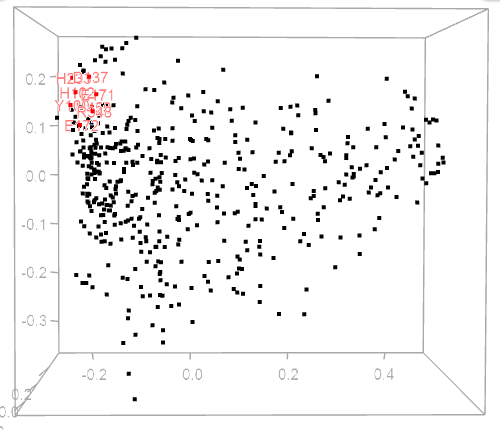
6. MDS scatterplot

   The MDS plot is automatically updated upon choosing a residue on a heatmap, circular diagram, or cladogram. Residues shown on a corresponding circular diagram will be highlighted on the MDA plot by red and residue labels.

   One can zoom the view using the mousewheel when hovering over the scatterplot or rotate the plot in 3D by dragging the mouse over the plot.

Example

Figure 1 illustrates how CoeViz can help identify functionally important residues using a peptidase from baker’s yeast (SwissProt ID: DUG1_YEAST) as an example. Dug1p is a Cys-Gly dipeptidase and belongs to the M20A family of metallopeptidases. The enzyme requires two Zinc ions in the active site to cleave the substrate. The structure of the enzyme is resolved (PDB ID: 4G1P), which makes it easier to map findings into 3D structure for illustration.

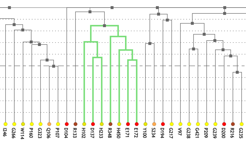
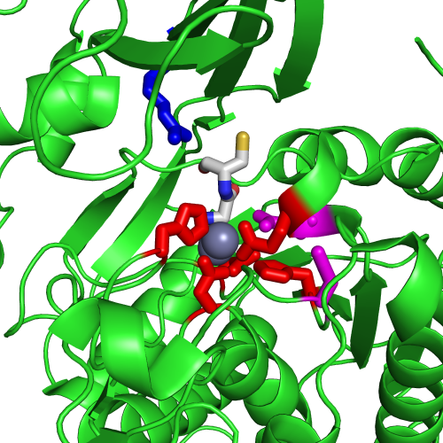
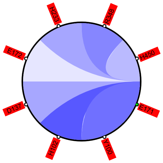
Figure 1A shows a fragment of the clustering tree based on χ2 scores weighted by phylogeny with the focus on the residues binding Zn (H102, D137, E172, and H450) and a catalytic residue (E171) that are clustered together. Interestingly, R348 is in the same cluster. When the residues are mapped to the resolved 3D structure, where the enzyme is co-crystallized with the substrate and Zn ions in the active site, R348 appears to be on the opposite side of the active site cavity and in contact with the substrate suggesting its role in substrate recognition and positioning the dipeptide into the catalytic center (Figure 1B). A circular diagram with the closest relationships to a given residue (e.g., E171) can be an alternative way for a quick identification of covarying residues (Figure 1C). In this view, all Zn binding residues are identified as the top co-varying residues with E171.

A
B	C
D	E
F	G
Figure 1. Example of using CoeViz to identify covarying amino acid residues and functionally related residues in the Dug1p Cys-Gly dipeptidase (PDB ID: 4g1p) as an example. A. The hierarchical clustering of residues based on χ2 scores weighted by phylogeny: a fragment of the overall cluster tree view with the focus on the selected Zn binding and catalytic residues. B. A 3D view at the catalytic site of the enzyme. Residues highlighted red (H102, D137, E172, D200, H450) are amino acids binding Zn (grey spheres); magenta – catalytic residues (D104, E171); blue is the residue involved in substrate recognition (R348). The substrate (Cys-Gly) is rendered as sticks colored by an atom type. C. A circular diagram showing residues with the closest relationships (χ2 ≥ 0.16) to E171 (highlighted with the green circle), one of the catalytic residues. D. A 3D multi-dimensional scaling scatterplot of co-variance matrix transformed into a distance matrix, with residues highlighted and labeled corresponding to those displayed on the circular diagram. E−G. Heatmap at different zoom levels (1, 3, and 7), representing pairwise χ2 scores. Blue cells indicate weak or no covariance; red cells show strong coevolution; intermediate shades are scores in between. Cells on the main diagonal, here, are individual probabilities: red are most frequent (p=1) and blue are least frequent (p=0).

Click on the buttons below to view interactive examples of using CoeViz to analyze baker's yeast metallopeptidase Dug1p (PDB ID: 4G1P).

Acknowledgements

For a complete list of people involed in related projects, software used, and funding, please visit the dedicated page.