POLYVIEW-MM: Documentation

POLYVIEW-MM Documentation

Index

About
Quick start
Data input
Motion-at-a-glance
Methods: Graphical 2D representation; Variability measurements; Identification of contacts
Integration with POLYVIEW-3D
Tips and tricks
Terms of use and disclaimer
Reference
Acknowledgements

Introduction

POLYVIEW-MM (Molecular Motion) enables animation of trajectories generated by Molecular Dynamics and related simulation techniques, as well as visualization of alternative conformers, e.g., obtained as a result of protein structure prediction methods or small molecule docking, using an intuitive web-based interface.

The server integrates high quality animation with structural annotation of molecular motions, and allows both qualitative and quantitative analysis of the results of macromolecular simulations. In order to facilitate structural analyses, POLYVIEW-MM combines:

interactive view and scripting-based conformational analysis using Jmol and its tailored extensions;
versatile annotation and publication quality animation using PyMol / POLYVIEW-3D;
motion-at-a-glance using customizable 2D summary plots of changes in secondary structure states and relative solvent accessibility of individual residues in proteins;
distance plots and analysis of intra- and inter-molecular contacts.

In addition, POLYVIEW-MM integrates visualization with various structural annotations, including automated mapping of known interaction sites from structural homologs, mapping of cavities and ligand binding sites, transmembrane regions, and protein domains.

Abbreviations used in this document

SS - secondary structure; SA - solvent accessibility; RSA - relative solvent accessibility; MD - molecular dynamics; PDB - protein data bank; NR - nuclear magnetic resonance; DSSP - dictionary of protein secondary structure (software).

Quick start

Specify a coordinate file with multiple models of the molecule, e.g., PDB code for a NMR structure with multiple models or a user generated file with MD trajectory snapshots
Select the type of motion analysis; currently available options include: MD or other trajectory; Morphs or distortions along normal modes; Protein-protein/DNA docking models; Protein-ligand docking models (for the latter, DLG or another PDB file with ligand poses needs to be specified)
Submit request to the server

Data input

At present, POLYVIEW-MM accepts the coordinate file in the PDB format with multiple models; trajectory files in the DCD format (used by NAMD and CHARMM), as well as the TRR format (GROMACS). DCD and TRR coordinate files are supposed to be accompanied by the structure definition files (PSF and GRO, respectively).
For the analysis of small molecule docking, the DLG format used by the popular AutoDock program is accepted as well.
Coordinate files derived from other MD programs should be converted to PDB or DCD or TRR files beforehand using, for example, CatDCD utility.
The file size should not exceed 50MB limit, otherwise the request will be rejected.
To reduce upload time, coordinate files can be submitted compressed by ZIP, GZIP, or BZIP2 (file extensions zip, gz, and bz2, respectively).
Trajectory analysis requires more computational resources and CPU time, so these requests will be sent to the cluster and queued. However, once analysis is concluded, further operations with images are processed interactively.
Optionally, an e-mail address can be specified to receive a link to view the results once the job is completed.

Multiple models are supposed to be defined using the PDB cards MODEL/ENDMDL (see example below).

MODEL        1                                                                  
ATOM      1  N   VAL A   1       0.965   0.298  -0.467  1.00  1.00           N  
ATOM      2  CA  VAL A   1       1.811   0.250  -1.701  1.00  1.00           C  
ATOM      3  C   VAL A   1       3.290   0.400  -1.320  1.00  1.00           C  
ATOM      4  O   VAL A   1       3.628   1.053  -0.346  1.00  1.00           O  
...
ATOM    407 HG23 ILE A  29      10.152   9.942 -22.140  1.00  0.00           H  
ATOM    408 HD11 ILE A  29      10.543  11.167 -18.839  1.00  0.00           H  
ATOM    409 HD12 ILE A  29       9.594  10.221 -17.693  1.00  0.00           H  
ATOM    410 HD13 ILE A  29      11.306  10.511 -17.391  1.00  0.00           H  
TER     411      ILE A  29                                                      
ENDMDL                                                                          
MODEL        2                                                                  
ATOM      1  N   VAL A   1       0.740   0.226  -0.858  1.00  1.00           N  
ATOM      2  CA  VAL A   1       1.662   0.223  -2.037  1.00  1.00           C  
ATOM      3  C   VAL A   1       3.117   0.317  -1.561  1.00  1.00           C  
ATOM      4  O   VAL A   1       3.411   0.923  -0.545  1.00  1.00           O  
...
ATOM    407 HG23 ILE A  29      10.809  10.803 -20.297  1.00  0.00           H  
ATOM    408 HD11 ILE A  29      11.414  10.731 -16.815  1.00  0.00           H  
ATOM    409 HD12 ILE A  29      10.441  12.035 -16.132  1.00  0.00           H  
ATOM    410 HD13 ILE A  29      10.422  10.438 -15.385  1.00  0.00           H  
TER     411      ILE A  29                                                      
ENDMDL                                                                          
...

Motion-at-a-glance

POLYVIEW-MM provides insights into molecular motion by enabling a quick analysis of conformational changes in terms of SS, SA/RSA (Figure 1), Phi/Psi angles (plain text only), protein-protein/DNA/ligand, as well as intra-molecular contacts (Figure 2). Several types of customizable 2D plots can be generated as described below.

The initial view of SS/RSA changes includes the following elements: residue numeration, amino acid sequence, corresponding variability measure, and SS states (or SA/RSA bins) encoded by colors. On top of it, a grid is placed for the easy tracking of changes along the extended trajectories. Each cell of the grid represents 10 residues in 10 consecutive models. Any element of the image mentioned above can be removed using a web-form accompanying the image. See examples in Figure 1, panels A-F. For initial visualization, all eight SS states are used (G, H, I, T, E, B, S, and C), but they can be optionally reduced down to three states (H, E, and C). See example in Figure 1, panel G.

Capturing changes in SS states
A	B

C	D

E	F

G	H

Capturing changes in RSA states
I	J

Figure 1. Examples of the different views of protein motion based on the ensemble of 25 NMR models (PDB code 1acw). A and I. Annotations produced with default settings after the initial data submission. B-F. Resulting images after hiding individual annotation elements described in the text above. G. View of motion after reducing the number of SS states (in particular, T and S were converted into C). H. Image after switching the variability measure to 8 states entropy. I-J. Motion in terms of SA changes, with variability measured by RSA and SA variances, respectively.

Capturing changes in contacts
A
B
C
Figure 2. Examples of different views of inter- (panels A, B) and intra-molecular (panel C) contacts. A. Analysis of the contacts between protein and ligand. The models were produced using a docking simulation. Files containing structures of the receptor and ligand poses are available for download from here ( receptor, ligand ), as well as from the home page of POLYVIEW-MM. As can be seen from the contacts summary, while the majority of poses were found energetically favourable near the residues 373-377 (NDLQT), one binding mode (model 5) indicates an alternative location of the ligand binding with low estimated energy (residues 335-337, TQT). B. Analysis of the interchain contacts for the first chain of a protein-protein complex obtained using a protein docking simulation. Example of the docking models is available here, as well as from the server home page. Frequency bars allow the user to quickly identify the residues of one chain most frequently observed in contact with the second chain. C. Analysis of the distance fluctuation between residues 1047 and 1151 (alpha carbons; atom IDs 2 and 1596, respectively) in the NMR-derived 3D structure of the nucleotide binding domain of the human Menkes protein (PDB ID: 2kmv). The chart shows high flexibility of the extended loop, as the distance from the tip of the loop (D1151.CA) to the N-terminus (S1047.CA) varies between 5.4 and 1.3 nm.

Methods

Graphical representation

Pictorial definitions used in POLYVIEW-MM for protein representation

Legend		Description
		Amino acid residue numeration
		Indicator of variability (for SS/RSA)
		0 - the least variable (rigid),
		9 - the most variable (flexible)
		Frequency of contacts
		0 - least observed in contact,
		9 - most frequent in contact
		Relative solvent accessibility (RSA)
		0 - completely buried (0-9% RSA),
		9 - fully exposed (90-100% RSA)

Secondary structure color codes

G	3-turn helix
H	4-turn helix
I	5-turn helix
E	extended strand
B	residue in isolated β-bridge
C	unstructured loop, coil
T	hydrogen bonded turn
S	bend
X	gap in structure

SS and SA are calculated using the DSSP program. To collect statistics on structural changes, eight (G, H, I, T, E, B, S, and C) and three (H, E, and C) SS states are used as defined in DSSP. RSA for a residue at a given position is SA normalized by the maximal value of the solvent exposed surface area for a given type of amino acid. Thus, RSA adopts values between 0 and 100%, with the latter corresponding to a fully exposed residue.

Variability measures

Per-residue variability of the abovelisted characteristics throughout trajectory is measured using the following statistics.

Entropy of SS: S = −K · ∑ p_i · log(p_i),
where K is a normalization factor K = 1 / log(N); N - number of SS states (8 or 3); p_i - probability of i-th state. This measure provides the insight as to how many SS states a given residue was involved in through the trajectory.
Counts of hoppings between SS states
This measure indicates how often a given residue changed its SS state through the trajectory.
Variance of SA and Variance of RSA: s² = 1/(n−1) · ∑(y_i − mean(y))²,
where n is the number of conformations in trajectory; y - respective SA and RSA observed at the sequence position i; mean(y) - the average value of SA (or RSA) for the i-th amino acid across all structural models. The first measure is more sensitive to minor changes in SA compared to variance of RSA.
Frequency of contacts
When analysis of protein-protein, protein-DNA, or protein-ligand docking models are requested, per-residue frequencies of being in intermolecular contact are computed throughout the models.

All measures are normalized to the corresponding maximums observed across all residues in one protein chain. All computed statistics are used in visualization and available for download in the plain text format.

Identification of contacts

Following previous studies, we define protein-protein interaction sites based on the RSA change upon complex formation, i.e. RSA difference between an unbound and bound (complex) structure of an individual chain. The procedure and thresholds used to assign an amino acid residue as an interaction site can be found in the SPPIDER documentation. Protein-protein interaction interfaces can be characterized in terms of the surface area buried upon complex formation, amino acid properties, and the presence of conserved hot spots, facilitating analysis of protein docking simulations, for instance.

Protein-ligand contacts are determined using the respective procedure adopted in Protein Explorer and subsequently in the FirstGlance in Jmol server (FGiJ) that accounts for hydrogen bonds, water and salt bridges, hydrophobic and aromatic ring interaction, and different types of metals binding. For the corresponding bond distance definitions, the reader is referred to the FGiJ documentation. Mapping specific residues in contact with the ligand in alternative poses of protein-ligand complexes can be used to assess the results of docking simulations. Consistency of interacting sites observed in protein-protein or protein-ligand docking models is measured by computing frequency of being in contact with the interacting co-factor.

3D Visualization

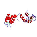
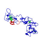
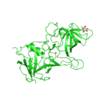
Interactive 3D visualization is provided using the Jmol java applet. It allows the user to animate a trajectory at different rate and access to a specific model. High quality animation is available via the link to POLYVIEW-3D provided at the resulting page. The images produced can be placed into PowerPoint slides or other electronic resources. No additional installation necessary for using both Jmol and POLYVIEW-3D. Figure 3 provides links to animations generated using different types of molecular simulations and deposited to the POLYVIEW gallery. Click on each thumbnail to view a full sized animation.

A	B	C

Figure 3. Examples of the different types of molecular motion. A. Animation showing the ensemble of NMR models for calmodulin indicates likely extent of conformational changes in solution. Backbone of the protein is rendered and colored according to SS states it adopts. B. MD trajectory for a resilin-like elastomeric peptide with Tyrosine side chains shown to underscore their propensity to be in contact. C. Alternative poses of the fucose ligand with respect to a Norovirus capsid protein obtained from the ligand docking simulation.

For the interactive analysis of conformational changes using Jmol, the following options are provided in addition to those built-in the Jmol applet and accessible via right-mouse click on the Jmol pane.

Browse models The user can review the structural models successively by using the buttons Next and Prev on the form. It is also possible to jump to a specific model by typing its number in the text field and pressing the button Jump to. The order number of the currently presented model is reflected at the Jmol pane at the top left corner. In addition, all models can be viewed simultaneously using the button Show all.

Animate models Available conformations of the submitted macromolecular structure can be visualized as animation using a single run through all models (button Once), endless loop starting each time from the first model (Loop), and endless reversible loop when models enumerated from the first to the last and backward, from the last to the first (Reversible Loop), with additional pauses at the terminal models. The rate of animation can be set in terms of frames per second (fps) using the corresponding text field.

Custom Jmol commands The user can manipulate Jmol in order to change/improve the structure rendering. Multiple commands separated by semicolon can be specified in the corresponding text field and then applied using the Apply button. The same can be achieved from the Java console, which is available from the context menu of the Jmol pane (right-mouse click). The syntax of the commands can be found in the Jmol documentation.

Highlighting Residues can be highlighted using colors with side chains rendered as sticks as opposed to the ribbon rendering of the overall atructure.

Available colors are red, green, blue, cyan, magenta, and yellow. Colors are specified by their corresponding first characters.
In case of macromolecules with multiple chains, a chain label for residues of interest needs to be specified as well.
Numbers of residues to be highlighted should be enumerated with comma delimitation (white spaces are ignored). The use of dashes to define a range of numbers is also supported.

The syntax of the string used to specify residues to be highlighted is the following: [Chain_label:]Residue_number[:Color], where '[ ]' denotes optional parts of the string. Capital letters R, G or B are used to highlight a residue in both color and bold font style, whereas lower case characters result in highlighting by the corresponding color only.

Below are several examples:
A:145:r - highlight the 145th residue in chain A using red color
C:5-10 - highlight residues from 5 through 10 in chain C using sticks to show their side chains
14-17,25-30,43:b - highlight residues 14, 15, 16, 17, 25, 26, 27, 28, 29, 30 in the first chain by showing side chains and blue color for a residue 43
A:3,A:10-20,A:35,B:15-20,B:25,B:40 - highlight residues 3, 10-20, 35 in chain A and residues 15-20, 25, 40 in chain B by showing their side chains.

To facilitate the conversion of the residue list to the required format, a separate web-form is provided via the link Converter on a resulting page.

Contact analysis This set of options appears only when Jmol successfully loads the macromolecular structure. The user can type in or click on a pair of atoms of interest to review the distance fluctuation between these atoms throughout the trajectory. Distance can be measured in angstroms, nanometers, and picometers. Distance fluctuation for a given pair of atoms can be retrieved either as a chart or in the plain text format. If multiple atom pairs were chosen, the data are retrieved for the last selected pair only.

Integration with POLYVIEW-3D

POLYVIEW-MM allows to display trajectories and multiple conformers using interactive animations and static views in Jmol, coupled with tailored selection and annotation options. These can be subsequently imported into POLYVIEW-3D in order to generate publication quality static pictures and animations using the PyMol rendering. The POLYVIEW-MM resulting page contains a link to POLYVIEW-3D that passes to the latter the coordinate file, current orientation of the structure in Jmol pane, and zooming factor.

All movies and plots generated by the server can be deposited with user-defined annotations to an image library as a mechanism to document and share data with colleagues. Details regarding the use of POLYVIEW-3D to generate high quality images and animations can be found in the POLYVIEW-3D tutorial.

Tips and tricks

Below are some tips that help make some tricks with the interactive Jmol view and images of protein annotations:

To apply new rendering and color settings in Jmol to all conformations (frames), there are two ways:
(1) For less experienced users, make right mouse click on the Jmol pane, choose item Model and click on All. When all models appear, apply any rendering/coloring options using the popup menu. Then, select some specific model via popup menu, or use Jump to button on the POLYVIEW-MM resulting page, which makes visible only specific model while keeping all changes made for other models.
(2) For more advanced users, open Jmol/Java console or use text field Custom Jmol command to type in and apply any rendering command using Jmol scripting language that will be applied to all models at the same time.
To accelerate the upload of the trajectory, use the file compression. Accepted formats are ZIP, GZIP, or BZIP2 (file extensions zip, gz, and bz2, respectively).
To convert a trajectory coordinate file to one of the accepted formats (DCD, TRR, or multi model PDB), use some convert utility, such as CatDCD or MDAnalysis. Additional documentation on the use of CatDCD can be found here.
To get an image in publishable format click on the tool Get as in the corresponding Image processing toolbar next to each image. You will be prompted to save a PS or TIFF file to a disk.
If a TIFF formatted image looks tiny, when embedded in a document, scale it to the desirable size, quality will not get worse.

Terms of use and disclaimer

All images generated by the POLYVIEW-MM server can be FREEly saved, printed, and distributed by means of any media without our written permission for academic and non-commercial purposes. However, the use of POLYVIEW-MM's pictures SHOULD be acknowledged by a reference to the server.

The use of the POLYVIEW web site and server is at your own risk and no liability is accepted for any loss or damage arising through the use of the web site and graphical representations generated by the server.

Reference

For citation, please use the following references:

A. Porollo, J. Meller (2010) POLYVIEW-MM: Web-based Platform for Animation and Analysis of Molecular Simulations, Nucleic Acids Research, 38, W662-W666.

POLYVIEW-MM: //polyview.cchmc.org/conform.html

Last update of the document: May, 2010
Back to the POLYVIEW-MM server home page