POLYVIEW-3D Tutorial
Part 5. Protein structure annotation settings
Index
- Pockets by CASTp
- Domains by Pfam
- TM segments by PDBTM
- Interacting sites
- Immune epitopes
- Interface by SPPIDER
- Interface by ConSurf
- Docking from CAPRI
- Molecular motions
These options include some of the most complex types of queries and structural analysis provided by POLYVIEW-3D. For example, they enable performing various structural and functional analyses, using both in house software, such as SPPIDER for the recognition of protein interaction interfaces, as well as several external servers, including CASTp for structural pockets identification, and ConSurf for assessment of evolutionary conservation. The results of these external resources are processed further (to a different degree) and combined with additional analysis performed by POLYVIEW-3D. One example is the ability to combine identification, prediction, and mapping of protein interaction interfaces performed by SPPIDER with the analysis of structural pockets identified by CASTp (and other topological features). See sections below for details.
There are two groups of settings within this options set. The first group invokes automatic requests to other web-servers and databases to obtain additional structural annotations. The second group uses precomputed results that were previously received (and possibly processed) from the other resources. In both cases, the resulting data is further processed by the POLYVIEW-3D server in order to yield 3D images of the macromolecular structures overlaid with the requested annotations, as described below.
Finding pockets using CASTp
This option sends an automated request to the CASTp server in order to perform a search for structural pockets within a given query protein. Identified pockets can be filtered by their area or volume. They are also automatically colored according to the CASTp color convention. Both atoms and residues constituting the corresponding cavities are listed as well. Pockets can also be optionally overlaid with the prediction of interacting sites automatically performed using the SPPIDER server. Pockets overlapping with predicted interfaces may represent potential targets for drug design and docking simulations.
Below is an example of a request to find pockets using CASTp, with pocket area cutoff of 100Å2. The structure of purine nucleoside phosphorylase in transition state was taken as a query structure (PDB id 1b8o).
| Pockets with surface area larger or equal to 100Å2 | |
|---|---|

|
|
| Click on respective image to see options used for its rendering. | |
Generated image is accompanied with the annotation table listing the residues located at each pocket.
| Pockets determined using CASTp (Show full version) | |||||||||
|---|---|---|---|---|---|---|---|---|---|
| Area, Å2 | Volume Å3 | Color |
Atoms (Residue name:Residue number:Atom:Chain) Residues (Chain:Residue numbers) |
||||||
| 37 | 460.6 | 543.9 | green |
Atoms: ALA:116:C:A ALA:116:CB:A ALA:116:N:A ALA:116:O:A ALA:117:C:A ALA:117:CA:A ALA:255:CB:A ... Residues: A:32 33 61 64 84 86 88 115 116 117 118 192 ... |
|||||
| 36 | 103.3 | 167.3 | blue |
Atoms: ARG:148:CA:A ARG:148:CB:A ARG:148:CG:A ARG:148:N:A ARG:158:NE:A ARG:158:NH1:A ... Residues: A:140 143 145 147 148 149 158 159 160 |
|||||
| 35 | 136.5 | 124.8 | cyan |
Atoms: ARG:101:NH1:A ARG:101:NH2:A ARG:148:O:A ARG:158:NH2:A ASN:151:CA:A ASN:151:OD1:A ASN:3:CB:A ASN:3:N:A ASN:3:OD1:A ... Residues: A:3 101 146 147 148 149 150 151 152 158 230 |
|||||
| 34 | 115.9 | 109.7 | yellow |
Atoms: ARG:210:CG:A ASN:121:C:A ASN:121:O:A GLY:119:C:A GLY:119:CA:A GLY:119:O:A LEU:120:C:A ... Residues: A:119 120 121 122 124 210 244 245 247 |
|||||
| 33 | 111.8 | 85.6 | magenta |
Atoms: GLN:273:CA:A GLU:272:C:A GLU:272:CA:A GLU:272:CB:A GLU:272:CG:A GLU:272:O:A ... Residues: A:38 41 73 272 273 275 276 |
|||||
| 31 | 103.8 | 80.5 | orange |
Atoms: ARG:101:CD:A ARG:101:CZ:A ARG:101:NE:A ARG:101:NH1:A ARG:101:NH2:A ASN:3:OD1:A ... Residues: A:3 10 94 97 98 101 146 227 |
|||||
| 29 | 101.5 | 44.2 | brown |
Atoms: GLU:224:OE2:A HIS:86:CA:A MET:194:CE:A MET:219:O:A MET:87:N:A PHE:85:O:A ... Residues: A:85 86 87 93 96 194 219 220 221 223 224 |
|||||
Mapping domains using Pfam
When this option is selected, POLYVIEW-3D performs a sequence homology
search using
BLAST
against the local version of
Pfam database.
Amino acid sequence used for query is derived from the
ATOM section of a PDB
file. If significant sequence homology
(E-value ≤ 0.001 AND
sequence identity ≥ 70%) is found to one or
more domains, they are mapped to the query structure
using distinct colors for each domain. Below is the
example of the annotated structure of ZAP-70
tyrosine kinase (PDB id 2ozo).
| Domains from Pfam | |
|---|---|

|
|
| Click on respective image to see options used for its rendering. | |
Generated image is accompanied with the annotation table listing the identified domains.
| Protein families found using Pfam (Show full version) | |||||||||
|---|---|---|---|---|---|---|---|---|---|
| Chain | Entry | Description | E-value | Color | Residues | ||||
| A | Domain Pkinase_Tyr |
Protein tyrosine kinase | 1e-140 | pink | PDB numbering 338 339 340 341 342 343 344 345 346... Amino acid sequence LIADIELGCG NFGSVRQGVY... |
||||
| A | Domain SH2 |
SH2 domain | 3e-39 | gold | PDB numbering 10 11 12 13 14 15 16 17 18 19 20 21 22... Amino acid sequence FFYGSISRAE AEEHLKLAGM... |
||||
| A | Domain SH2 |
SH2 domain | 6e-38 | purple | PDB numbering 163 164 165 166 167 168 169 170 171... Amino acid sequence WYHSSLTREE AERKLYSGAQ... |
||||
Mapping putative TM segments using PDBTM
Upon request of this option, POLYVIEW-3D makes search in the local copy of the
PDBTM
database of putative trans-membrane segments. Specifically,
it performs a sequence homology search using
BLAST.
Amino acid sequence used for query is
derived from the ATOM section
of a PDB file. If significant sequence homology
(E-value ≤ 0.001 AND
sequence identity ≥ 70%) is found to one or
more proteins, the best matching homolog is taken. Images
below demonstrate the annotation on membrane spanning segments
as determined in PDBTM using the TMDET
automated algorithm (for details, please refer to the
original papers).
The structure of Catalytic Core (Subunits I and II) of
Cytochrome c oxidase from Rhodobacter sphaeroides
serves as an example of alpha-helical TM protein (PDB id
2gsm), whereas the structure of the
sucrose-specific porin ScrY (PDB id 1a0s) from
Salmonella typhimurium represents beta-barrel TM
proteins.
| TM segments from PDBTM Alpha helical |
TM segments from PDBTM Beta barrel |
|---|---|

|

|
| Click on respective image to see options used for its rendering. | |
Generated image is accompanied with the annotation table listing the TM spanning regions (if any found).
| Trans-membrane domains found using PDBTM (Show full version) | |||||||||
|---|---|---|---|---|---|---|---|---|---|
| Chain | PDBTM (Type) |
E-value | Residues in the membrane spanning regions | ||||||
| A | 1m56 (Alpha) |
0.0 | PDB numbering 33 34 35 36 37 38 39 40 41 42 43 44 45 46 47 48 49 50 51 52 53= 104 105 106 107 108 109 110 111 112 113 114 115 116 117 118 119 120 121 122 123 124= ... Amino acid sequence YLFTGGLVGLISVAFTVYMRM= ILMMFFVVIPALFGGFGNYFM= ... |
||||||
| B | 2gsm (Alpha) |
0.0 | PDB numbering 61 62 63 64 65 66 67 68 69 70 71 72 73 74 75 76 77 78 79 80= 100 101 102 103 104 105 106 107 108 109 110 111 112 113 114 115 116 117= Amino acid sequence ILVIIAAITIFVTLLILYAV= LEIAWTIVPIVILVAIGA= |
||||||
| Trans-membrane domains found using PDBTM (Show full version) | |||||||||
|---|---|---|---|---|---|---|---|---|---|
| Chain | PDBTM (Type) |
E-value | Residues in the membrane spanning regions | ||||||
| P | 1a0s (Beta) |
0 | PDB numbering 77 78 79 80 81 82 83 84 85= 117 118 119 120 121 122 123= 138 139 140 141 142 143 144 145 146 147 148 149 150 151 152 153= ... Amino acid sequence GYARSGVIM= TYVEMNL= KVMVADGQTSYNDWTA= ... |
||||||
| Q | 1a0s (Beta) |
0 | PDB numbering 77 78 79 80 81 82 83 84 85= 117 118 119 120 121 122 123= 138 139 140 141 142 143 144 145 146 147 148 149 150 151 152 153= ... Amino acid sequence GYARSGVIM= TYVEMNL= KVMVADGQTSYNDWTA= ... |
||||||
| R | 1a0s (Beta) |
0 | PDB numbering 77 78 79 80 81 82 83 84 85= 117 118 119 120 121 122 123= 138 139 140 141 142 143 144 145 146 147 148 149 150 151 152 153= ... Amino acid sequence GYARSGVIM= TYVEMNL= KVMVADGQTSYNDWTA= ... |
||||||
Mapping interaction sites from PDB complexes using SCORPPION
With this option, one can retrieve information about all interaction sites found among close sequence homologs deposited in PDB. Search is automatically performed using the SCORPPION server. Interaction sites are the residues in contact with other protein chains, DNA or RNA, or ligands. Different types of interactions, as well as their combinations are colored distinctly. Interaction sites can be optionally contrasted with protein interfaces predicted by SPPIDER.
Below is example of mapping different types of interactions from the close sequence homologs to the structure of transcription factor CSL (PDB id 1ttu, chain A).
| Interfaces by SCORPPION | |
|---|---|

|
|
| Click on respective image to see options used for its rendering. | |
Generated image is accompanied with the annotation table listing residues involved in intermolecular interactions.
| Interacting sites mapped from homologs (Show full version) | |||||||||
|---|---|---|---|---|---|---|---|---|---|
| Chain | Type of contact | Residues | |||||||
| A | P−DNA | 226 227 229 230 231 232 233 234 235 236 237 334 366 367 368 369 370 371... | |||||||
| A | P−Protein | 223 281 282 285 287 289 294 298 299 301 319 338 339 340 342 346 348 350... | |||||||
| A | P− Protein/DNA |
337 | |||||||
Mapping linear immune epitopes from IEDB
This option allows the user to map all linear Ab- and MHC-targeted epitopes currently known for a submitted protein or its close sequence homologs. Immune Epitope Database (IEDB) is employed to retrieve information about epitopes. Mapping is performed based on sequence homology. Peptides with at least 70% sequence identity are considered as putative matches. Multiple matches are clustered by their location in the target sequence extending the boundaries of each cluster to the longest match. In addition, average relative solvent accessibility (RSA) is computed for a given match that allows to evaluate burial state of identified peptides within the structure. Based on observations in PDB, peptides with the average RSA below 40% most likely represent MHC epitopes, as they become accessible upon protein degradation. Epitope mapping can be overlaid with other annotations available at POLYVIEW-3D, e.g., with protein-protein or protein-ligand binding sites. Such a combined annotation facilitates the inference of functional implications for a given antibody-antigen binding.
Below is an example of the mapping of different types of epitopes (linear and conformational) based on sequence data from IEDB and automated structure analysis performed by POLYVIEW-3D for ribonuclease A (RNase A). In this case, the peptide colored pink is a MHC epitope; yellow is an Ab epitope; red is a conformational Ab epitope identified using the 3D structure (biological unit) PDB ID 1bzq.
| Immune epitopes by IEDB | |
|---|---|

|
|
| Click on respective image to see options used for its rendering. | |
Generated image is accompanied with the annotation table listing the identified epitopes.
| Peptidic epitopes found using IEDB | |||||||||
|---|---|---|---|---|---|---|---|---|---|
| Chain | Epitope IDs, Epitope match (Sequence identity, %) |
Color | Residues* | ||||||
| A |
108593
PVNTFVHESLADVQA (100) 124828 VNTFVHESLADVQA (100) 108594 PVNTFVHESLKDVQA (93) 108591 PVNTFVHEALADVQA (93) 108592 PVNTFVHESAADVQA (93) 108586 PVNAFVHESLADVQA (93) 108587 PVNTAVHESLADVQA (93) 108584 PVATFVHESLADVQA (93) 108590 PVNTFVHASLADVQA (93) 108588 PVNTFAHESLADVQA (93) 108589 PVNTFVAESLADVQA (93) |
pink |
Matching peptide PVNTFVHESLADVQA PDB numbering 42 43 44 45 46 47 48 49 50 51 52 53 54 55 56 Average RSA 27% |
||||||
| A |
130980
NCAYKTTQANK (100) |
gold |
Matching peptide NCAYKTTQANK PDB numbering 94 95 96 97 98 99 100 101 102 103 104 Average RSA 38% |
||||||
In case of complexes, RSA values refer to an 'unbound' state of the protein chain.
Average RSA below 40% indicates that the peptide is more likely to be a MHC-targeted epitope.
RSA above 40% may represent both Ab and MHC epitopes.
| Interface analysis | |||||||||
|---|---|---|---|---|---|---|---|---|---|
| Chain | Interface SA*, Å2 | HP index** | Residues | ||||||
| A | 568 | 0.59±0.74 | 59 60 61 62 64 68 69 70 71 73 76 111 112 115 | ||||||
| L | 557 | 0.91±0.85 | 1027 1028 1029 1031 1032 1099 1100 1101 1104 1106 1107 1109 1110 | ||||||
** HP -- hydrophobicity
Predicting protein interface using SPPIDER
This setting belongs to the second group of options that utilize
pre-computed results, which were received prior to
submitting a query to POLYVIEW-3D. The SPPIDER server
optionally generates a PDB file with temperature factor
fields modified according to the probability of that
residue to be involved in protein-protein
interactions. These files can be submitted to the
POLYVIEW-3D server as custom PDB files with
chain of interest to be colored using the
By B-factors color
scheme (see
Chains rendering settings).
Two examples below illustrate the use of POLYVIEW-3D to visualize
predictions by SPPIDER of interaction sites within the CSL
transcription factor (PDB id 1ttu, chain A). The
predictions are encoded using either classification or
regression approach (with a binary class assignment in the
first case, and a probability of being within an
interaction interface in the latter case, respectively),
and incorporated in the corresponding B-factor
fields. Color scheme applied is
By B-factor and described
in Chains rendering settings
section. Modified PDB files, used here for the images, are
also available for download
(classification-based and
regression-based
prediction).
| Interfaces by SPPIDER as classification |
Interfaces by SPPIDER as regression |
|---|---|

|

|
| Click on respective image to see options used for its rendering. | |
Generated images are accompanied with lists of residues that are grouped either by class assignment or in probability bins (see the corresponding tables below).
| Interface prediction using SPPIDER as classification (Show full version) | |||||||||
|---|---|---|---|---|---|---|---|---|---|
| Chain | Class | Residues | |||||||
| A | Positive | 230 399 400 401 402 403 412 413 415 416 419 426 428 429 430 431 432 433 435 436 ... | |||||||
| A | Negative | 195 196 197 198 199 200 201 202 203 204 205 206 207 208 209 210 211 212 213 214 ... | |||||||
| Interface prediction using SPPIDER as regression (Show full version) | |||||||||
|---|---|---|---|---|---|---|---|---|---|
| Chain | Probability, % | Residues | |||||||
| A | 90-100 | 403 467 572 573 574 | |||||||
| A | 80-89 | 402 413 431 433 463 464 570 575 576 578 622 | |||||||
| A | 70-79 | 400 401 412 416 436 440 458 516 519 557 571 577 626 655 | |||||||
| A | 60-69 | 230 415 429 430 437 439 556 660 | |||||||
| A | 50-59 | 399 419 426 428 432 435 441 442 462 466 512 569 631 632 654 659 | |||||||
| A | 40-49 | 231 233 391 398 406 407 411 414 443 465 502 515 517 567 568 612 617 623 ... | |||||||
| A | 30-39 | 195 229 234 319 328 354 389 397 404 405 409 410 434 438 445 447 456 460 ... | |||||||
| A | 20-29 | 232 235 243 245 259 262 280 281 285 297 320 329 377 378 388 390 418 420 ... | |||||||
| A | 10-19 | 196 197 199 205 207 208 211 212 220 226 227 237 247 250 252 254 255 258 ... | |||||||
| A | 0-9 | 198 200 201 202 203 204 206 209 210 213 214 215 216 217 218 219 221 222 ... | |||||||
Finding functional regions using ConSurf
The ConSurf server ranks residues according to their relative conservation scores that can be used for the identification of putative functional regions within a given structure. The server also modifies the original PDB file to encode conservation scores by replacing B-factor fields. Such a file can be submitted to POLYVIEW-3D. Then, by specifying the chain of interest to be colored by B-factors, one can obtain high-quality images of ConSurf results using its original color scheme.
Below is example of the ConSurf output, with conservation scores
encoded as B-factors and residues colored using the
ConSurf color scheme. The same protein was used as in the
previous section (PDB id 1ttu, chain A). Color
scheme applied is
By B-factor and described
in Chains rendering settings
section. PDB file modified by the ConSurf server and used
for the image is also available for
download.
| Functional regions by ConSurf | |
|---|---|

|
|
| Click on the image to see options used for its rendering. | |
Generated image is accompanied with the annotation table listing the residues binned by the ConSurf conservation scores.
| Relative amino acid conservation using ConSurf (Show full version) | |||||||||
|---|---|---|---|---|---|---|---|---|---|
| Chain | Color | Residues | |||||||
| A | 9 | 199 203 221 222 223 224 225 226 227 228 231 232 233 234 238 239 240 300 327 328... | |||||||
| A | 8 | 198 229 230 235 237 241 243 244 248 291 302 319 330 341 343 356 358 384 385 389... | |||||||
| A | 7 | 219 249 288 290 295 340 387 390 393 419 422 460 465 479 483 490 511 515 516 517... | |||||||
| A | 6 | 208 209 252 257 258 259 260 261 262 280 281 282 283 284 292 298 301 362 371 379... | |||||||
| A | 5 | 214 220 236 246 293 294 304 320 331 335 348 350 352 376 413 416 423 440 444 448... | |||||||
| A | 4 | 202 206 207 289 325 424 435 449 450 461 482 499 506 518 523 573 585 636 | |||||||
| A | 3 | 211 216 250 285 299 345 346 347 355 441 445 453 459 502 512 529 551 578 588 591... | |||||||
| A | 2 | 287 303 321 324 354 454 480 505 522 535 569 596 603 622 629 630 632 | |||||||
| A | 1 | 195 196 197 200 201 204 205 210 212 213 215 217 218 242 245 247 251 253 254 255... | |||||||
Analysis of docking models from CAPRI
POLYVIEW-3D provides an option for analyzing the docking models in the
CAPRI format
obtained by different programs or web-servers for
protein-protein docking. In addition to visualization of
docking models, POLYVIEW-3D performs their analysis and
assessment. In particular, when a custom PDB file with multiple
models of a protein complex (e.g., generated by the
ClusPro
server) submitted to POLYVIEW-3D using the
Docking models option, it
triggers SPPIDER predictions to perform for all chains
in the model. Unbound structures of these chains are used to
predict putative interaction interfaces, which are then
compared to the interfaces observed in each model. The
fraction of residues within the interface in a given model
that overlaps with SPPIDER predictions (averaged over both
chains) provides a simple score to rank these models. In
addition, the surface area and average hydrophobicity for
each interface within these models are computed to provide
a basis for further analysis and model ranking. Models can
be then re-ranked according to these values and sent to
refine image rendering.
The table below includes the output of the POLYVIEW-3D assessment of docking models for the system used as CAPRI target #9, and described in more details in Example 2 of the Advanced examples section. The two chains were submitted to the ClusPro server, in order to obtain 10 best ranking models of the protein complex (download results). The option for model assessment had been invoked by requesting the overlay with protein interfaces predicted by SPPIDER. NOTE: table rows (and thus different models) can be easily re-ordered (sorted) according to measures presented in the columns. In addition, the resulting page provides options to alter the sensitivity used to identify interaction sites from the SPPIDER initial (default) definition. It allows the user to make the interface overlap measure either more restrictive or loose.
| Analysis of docking models (Click on the header of column to re-sort models) |
|---|
| Model | Image | (1) ASA, Å2 |
(2) HP index |
(3) Overlap, % |
Chain A Interface ASA, Å2 |
Chain A Interface HP |
Chain B Interface ASA, Å2 |
Chain B Interface HP |
Residues at the interface (Overlap with SPPIDER prediction, %) |
|---|---|---|---|---|---|---|---|---|---|
| 1 | 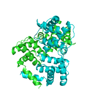 |
2436 | 1.04 | 52.42 | 1246 | 1.06±0.72 | 1190 | 1.01±0.72 |
Chain: A (54.84%) Overlapped: 2 3 5 6 7 9 ... Observed: 21 37 46 63 112 ... Predicted: 1 4 8 12 13 14 ... Chain: B (50.00%) Overlapped: 2 3 5 6 7 9 ... Observed: 21 37 38 46 ... Predicted: 1 4 8 12 13 14 ... |
| 2 | 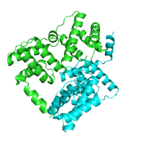 |
2150 | 0.72 | 45.69 | 1081 | 0.68±0.67 | 1069 | 0.75±0.67 |
Chain: A (41.38%) Overlapped: 1 2 3 6 41 ... Observed: 34 36 37 38 112 ... Predicted: 4 5 7 8 9 10 ... Chain: B (50.00%) Overlapped: 1 2 3 6 41 ... Observed: 34 36 37 38 ... Predicted: 4 5 7 8 9 10 ... |
| 3 | 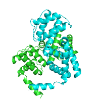 |
2438 | 0.95 | 32.73 | 1218 | 0.95±0.73 | 1220 | 0.95±0.74 |
Chain: A (32.14%) Overlapped: 5 8 9 12 49 53 59 61 134 Observed: 62 63 65 66 ... Predicted: 1 2 3 4 6 7 ... Chain: B (33.33%) Overlapped: 5 8 9 12 49 53 59 61 134 Observed: 62 63 65 66 67 96 97 ... Predicted: 1 2 3 4 6 7 ... |
| 4 | 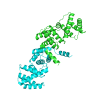 |
2091 | 0.96 | 47.22 | 1050 | 0.98±0.67 | 1041 | 0.95±0.67 |
Chain: A (44.44%) Overlapped: 3 7 10 11 15 17 18 40 Observed: 21 25 28 29 32 ... Predicted: 1 2 4 5 6 8 9 ... Chain: B (50.00%) Overlapped: 3 7 10 11 15 17 ... Observed: 21 25 28 29 32 ... Predicted: 1 2 4 5 6 8 9 ... |
| 5 | 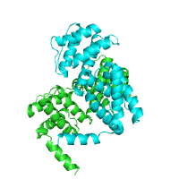 |
2374 | 1.02 | 21.45 | 1176 | 1.00±0.74 | 1198 | 1.03±0.73 |
Chain: A (22.22%) Overlapped: 53 59 61 134 137 139 Observed: 62 63 65 66 67 69 ... Predicted: 1 2 3 4 5 6 7 8 ... Chain: B (20.69%) Overlapped: 53 59 61 134 137 139 Observed: 62 63 65 66 67 69 ... Predicted: 1 2 3 4 5 6 7 8 ... |
| 6 | 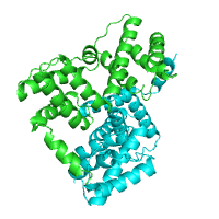 |
2479 | 0.83 | 48.34 | 1253 | 0.88±0.69 | 1226 | 0.79±0.69 |
Chain: A (51.52%) Overlapped: 1 2 3 6 7 40 41 ... Observed: 21 28 31 32 33 34 ... Predicted: 4 5 8 9 10 11 12 ... Chain: B (45.16%) Overlapped: 1 2 3 6 10 40 146 ... Observed: 31 32 33 34 36 37 ... Predicted: 4 5 7 8 9 11 12 ... |
| 7 | 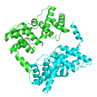 |
1276 | 0.79 | 46.05 | 634 | 0.80±0.69 | 642 | 0.77±0.70 |
Chain: A (50.00%) Overlapped: 1 2 3 5 6 10 41 ... Observed: 36 161 163 174 177 ... Predicted: 4 7 8 9 11 12 ... Chain: B (42.11%) Overlapped: 1 2 3 5 6 10 ... Observed: 36 161 162 163 ... Predicted: 4 7 8 9 11 12 ... |
| 8 | 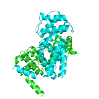 |
2305 | 1.02 | 30.81 | 1165 | 1.00±0.69 | 1140 | 1.04±0.69 |
Chain: A (29.63%) Overlapped: 6 53 56 58 59 61 134 139 Observed: 62 63 64 66 67 69 ... Predicted: 1 2 3 4 5 7 8 9 ... Chain: B (32.00%) Overlapped: 6 53 56 58 59 61 134 139 Observed: 63 64 66 67 114 115 ... Predicted: 1 2 3 4 5 7 8 9 ... |
| 9 | 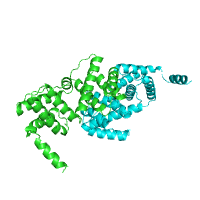 |
2081 | 0.89 | 51.47 | 1056 | 0.86±0.71 | 1025 | 0.91±0.70 |
Chain: A (50.00%) Overlapped: 144 147 151 154 165 ... Observed: 150 158 162 163 164 ... Predicted: 1 2 3 4 5 6 7 8 9 ... Chain: B (52.94%) Overlapped: 144 147 151 154 165 ... Observed: 150 158 162 163 164 ... Predicted: 1 2 3 4 5 6 7 8 9 ... |
| 10 | 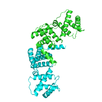 |
2059 | 1.12 | 51.19 | 1032 | 1.11±0.67 | 1027 | 1.13±0.66 |
Chain: A (52.38%) Overlapped: 3 6 7 10 11 15 17 ... Observed: 21 25 28 29 32 33 ... Predicted: 1 2 4 5 8 9 12 13 ... Chain: B (50.00%) Overlapped: 3 6 7 10 11 15 17 ... Observed: 21 25 28 29 31 32 33 ... Predicted: 1 2 4 5 8 9 12 13 ... |
1 − Total solvent accessibility buried upon complex formation
2 − Mean hydrophobicity index of the interfaces
3 − Average overlap across chains between observed interfaces in a given model and predicted by SPPIDER
Annotation of residues:
Overlapped(Red) - observed and predicted to be at the interface
Observed(Blue) - located at the interface in a given model, but not predicted
Predicted(Yellow) - predicted to be at the interface, but not observed in a model
Animation of macromolecular movements
There are a number of programs and web-servers performing simulation
and analysis of macromolecular movements, for example
Analysis of Dynamics of Elastic Network Model
(AD-ENM) or
Database of Macromolecular Motions
(MolMovDB).
Motion trajectories and structural distortions may help
identify flexible and rigid regions, localize
hinges and stable domains. In this regard, POLYVIEW-3D
has a function that analyzes trajectory
quantitatively and produces both animations and
2D-trajectory images. In order to invoke this function,
the user has to chose the option
Trajectories and distortions
and submit a PDB-formatted
coordinate file with conformational changes recorded as
models.
NOTE: When this structure annotation is requested,
POLYVIEW-3D ignores the current setting of the
Type of request option in the
Image Settings
field set. In contrast to the option that animates
Models
from the Animation settings,
this option generates a movie comprising of all available
models and makes the motions reversible. Images shown
below represent two macromolecular motions as deduced by the
corresponding servers. Coordinate files were taken from
the examples available at those servers and can be downloaded here:
AD-ENM example of myosin deformation,
MolMovDB example of calmodulin hinge motion.
| Low-frequency motion by AD-ENM | Morph by the Morph Server |
|---|---|

|

|
| Click on respective image to see options used for its rendering. | |
Along with animation, the resulting page presents 2D-plots with trajectories of structural changes in terms of secondary structure (SS) and relative solvent accessibility (RSA), and with per-residue analysis of protein flexibility. The details on the measures used to quantify conformational changes as well as the options to customize a 2D-plot can be found in the POLYVIEW-MM documentation. Below are 2D-plots produced for SS and RSA changes occurring during the calmodulin hinge motion as interpolated by the Morph Server.
| Conformational changes in calmodulin in terms of SS |
|---|
|
| Conformational changes in calmodulin in terms of RSA |
|
Last modified: Thu Feb 9 13:28:25 EST 2012